GIS Programming: Building Script Tools

       Good day Python and GIS enthusiasts. This weeks work is dedicated to taking stand alone scripts and making them into Script Tools usable within ArcMap. The overall objectives were to learn about and exercise these script to tool skills. There are many reasons that you may want to utilize a Script Tool which takes a script and modifies it for use within the geoprocessing environment over a stand alone script which is usually ran in a Python user interface. One of the biggest advantages is the use of specific parameters. A Script Tool allows you to more easily select the inputs and outputs you desire over having to change copious amounts of variables and hard coded file paths. There is less need to build in error checking as parameters assigned to a script tool are all of a certain type. The tool wont let you use parameters that don't match the needed type, whereas you could be stuck digging through a long error message in the stand alone. Tools are integrated with the environment you already have built for whatever processes you're working with in ArcMap. Tools can be packages and shared more readily than some standalone scripts, especially if the person you're sending the script to has little to no knowledge of Python. So with all of that said, lets look at a quick rundown of transforming a stand alone script to a Script Tool, and show some examples.
       First to build the tool you should be starting with a particular script executing whatever flavor of geoprocessing as you need. Then you need to start the transformation process. One of the biggest steps in this is changing hard coded file paths and entered parameters such as specific inputs and outputs to ArcMap and arcpy usable code. This takes the form of the GetParameter or GetParameter as text functions in arcpy. So as mentioned above we take the long string file path and replace with Variable = arcpy.GetParameter(index#), remembering that the parameter in the script needs to match the one you set up in your script tool. Now we need a place to house our script tool. This requires a custom tool box, new or previously established doesn't matter. But it cant be one of the default ArcMap toolboxes. Add a script to the tool box, Name it, label it, and slap a location to the script you're building the tool from on it.  If you're ready you can enter your specified parameters now, or finish the script tool creation without them and edit them later. A Script Tool without parameters assigned will still run like a standalone script. But, parameters are better, so lets input them corresponding to what we modified in our script, keeping a good index, and making sure our parameter types are good to go. Once this is accomplished your Script Tool is born.

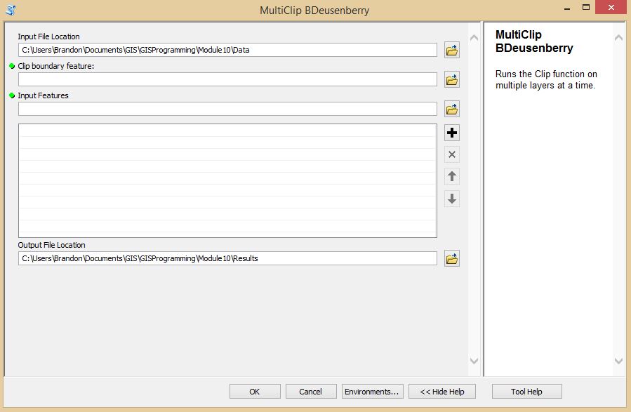
Above is a look at the Script Tool created for the assignment. If you're thinking it looks just like every other tool you've seen then congratulations to me, thats the point. As mentioned above though, you have basically free reign of the parameters you want to choose. This tool clips multiple features to a specified feature at once. So you can see where you have control of the parameters.

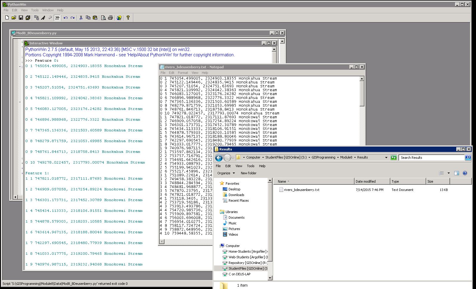
      After having built the Script Tool above we can run it like any other. However one of the cool features of a script tool over a stand alone is the ability to include messages within the geoprocessing environment, in this case the pop up tool progress box, and results window. With the standalone we typically only have the Pythin Interactive window available to us. 

Here is a good look at the results from having run the tool. You can see the messages mentioned above which have been generated in the progress window, and you can see the resulting shapefiles in the ArcCatalog look on the right, as well as the toolbox and script tool that were in use. 

      All in all it is hugely beneficial being able to transform a script to a script tool for use in ArcMap. And the last thing ill touch on is that this whole thing is shareable. Take the toolbox.tbx seen there in the image, and the script that generated it, zip them together using your favorite zip service, I like 7 Zip, and share away. Thank you for your time.

GIS Programming: Working with Rasters

Hello and welcome to week 9 of my GIS Programming class. This week is dedicated to working with rasters via python. The overall objectives of this week were to be able to list and describe rasters, and use raster objects in geoprocessing. Also, map algebra operators and classes for defining raster parameters were discussed.  The raster work also involved much interaction with the spatial analyst extension through arcpy.  The exercise and assignment culminated in a script producing the below result.

Above you can see the end result of the script, as well as the message traffic describing each step of the process  in the PythonWin interactive window. The pictured raster shows you two different areas, the green areas match a set of criteria established by the script. The black areas represent those that do not meet the prescribed criteria. To get this finalized image 5 different rasters were created then merged with map algebra. the 5 individual rasters set up certain particular criteria. A landuse raster was used to isolate forested areas using the remap and reclassify tools. Also, an elevation raster layer was used to create 4 specific rasters using the Slope and Aspect functions. I needed to identify slope areas between 5 and 20 degrees, and aspect areas between 150-270 degrees. These combined with the forested areas using the & operator generated this raster. The 5 individual rasters were all created on a temporary basis through working with arcpy. The save function was used with the final raster to allow it to be a permanent raster dataset. This is a handy feature because it allows all of the intermediate data to not clog up your various save locations, and only keep that which you specifically desire.
This kind of work with rasters is particularly useful for suitability analysis, and thats exactly what the above script mirrored. Taking multiple criteria and combining them to show a suitable area for whatever you need. This was a great foundation for working with rasters in arcpy.

GIS Programming: Work with Geometries

Greetings GIS and Python enthusiasts,
      Welcome to this weeks GIS programming excursion delving deeper into geometries. We are looking specifically at referencing and manipulating vector based geometry objects using python. Some of the bigger portions of this assignment involved taking data in a text file, ie coordinate information, and building a feature class from it. Or taking existing features and retrieving their geometry data and writing the information to a text file.  The basic tools to interact with these geometry objects have already been looked at previously, however we are expanding into concepts and items like geometry tokens as shortcuts for accessing the properties of a geometry object, or expanding on previously learned for loops by creating nested for loops to go multiple layers deep into a features properties by using a cursor object.
The actual assignment for this week revolved around taking a known polyline feature class and extracting information for each features vertices, ID, name of the feature, etc and writing it to a newly created text file.  Lets look at a combined picture of the outcome and then discuss some of the other specifics.

This is a look at multiple windows active at once containing both the interactive python window, after having the finalized script ran, a snippet of the text files results, and showing the created file itself. Some of the keys that made this script work were the nested for loop that was alluded to above, and specific code to write the output to the file in the manner that is shown. What are nested for loops? These are used to iterate over many different levels of geometry characteristics. Think of a feature as a combination of objects, I can ask a question about the feature as a whole, or perform an action on multiple features with a simple for loop. Lets say I need to look at some of the composite parts that make up a particular feature, like a set of vertices that make up a polyline or polygon, then I need a loop to reference the set of features, and a loop within this one to reference the items making up the feature. These loops within loops are referenced as nested. You can see in the screens above that each feature is shown with its vertices labeled 1 through however many for more simplification.
The hardest part of this lab came not from the nesting, or from getting the vertex information to display, but the simple OID which is the identified for the individual features (first character in the results screen), and the NAME field at the end. The OID, NAME, and a shape token were referenced in a cursor object as a list of features. I tried to use the same input method and code in the cursor variable to have the OID and name written to the text file. Long story short, what I was doing was trying to combine (concatenate) list objects and string objects. Python repeatedly told me no, this isnt possible. My initial flawed troubleshooting was working with brackets because I thought reorganizing these held the key. What I had realistically walked right over was the fact that I had already defined these list object in the cursor variable. I did not need to reuse them when telling python to write them to a text file. I needed to tell python to reference the list I already created and pull the value from there. This was a huge epiphany. Why recreate an object that I already have available for reference. This was the big thing I learned this week working with geometries. Thank you python! 

Applications in GIS: Local Government

Welcome to a continued look at GIS applications involving local government. The focus of this week is on parcel presentation and parcel editing. The goals of this weeks lab were to utilize county property appraisal data to create a parcel report, create a parcel map book, and edit and locate parcels based on specific criteria.  The appraisal data was used to identify specific attributes pertaining to the parcel, such as parcel ID, size, location, currently assigned zoning, etc.  The parcel map looks at a central parcel of interest as well as all adjacent parcels within .25 miles, using data driven pages to create an index viewing the area in segments (pages).
The initial steps of the lab continued last weeks participation activity exploring county appraisal information. The particular parcel of interest happens to belong to Mr Danny Zuko himself, and we used it as the basis for the map below.

This is just one of the 16 pages created through the use of Data Driven Pages (DDP). DDP is a particularly useful utility when needing to create many different pages of the same map. In this particular frame we are looking at page 10 of 16, which is index number C4. Looking at the bottom right of the page you can see the index overview, with the current page highlighted. Essentially this setup is done by creating an index layer which is built around a base layer. In this case the parcels within .25 miles described above are the base, and the index is created around it at a base scale of 1:2400.The yellow highlights the Zuko parcel. I adjust the base scale to one that has just enough overlap to provide better continuity from one map slide to another. I ended up using a 1:3000 scale. You can see the black lines indicate the different Index boxes, so you have slight overlap with the adjacent cells. The numbers in each of the parcels correspond to the attached map key which is labeled in a table based parcel report (not included). The report was based off of the attribute data table for the parcel layer. The hardest part of the parcel report was adding the zoning data which was not originally included by parcel. The zoning data while boring browns in this map are symbolized by all available zones shown in the legend in the upper right.
After the map book was complete the next portion of the assignment was to combine two parcels, then divide them again using different criteria. Then afterward create a search based on all parcels belonging to a particular owner, and analyzed according to size. The key tasks here were to utilize the data editor and merge the original parcels, then use the feature construction toolbar in conjunction with the editor to create a new parcel from the whole of the merged one. Several useful drawing tools were explored in this activity revolving around measuring distance, drawing parallel to other features, and drawing new line segments based on degree measurements.
This was an excellent continuation of looking at local government data from property data available on county GIS sites to what can be done with it in ArcMap. This was a good look at the tasks actually performed by some GIS analysts daily. Thank you.

Apps In GIS: Participation & County Appraising

Welcome to my participatory assignment overview for Application in GIS, focusing on some aspects of the wonderful information provided by county appraisers. Here We will look at some variations of information provided by my local county appraiser for Santa Rosa County Florida. Then we will look at some of the unique tasks that county appraisers often find themselves doing in the realm of GIS. Below I will reference some specific questions that guided the exploration of my county appraisers services.

1. Does your property appraiser offer a web mapping site?

Yes, the county appraisers website is linked in with the county main webpage which has a dedicated GIS map. The county appraisers features on the map offer parcel look up, sale information, tax information, and many other features.

County Appraisers website: http://www.srcpa.org/index.html
County GIS Home Site: http://www.santarosa.fl.gov/gis/#
Good link to the appraisal map services can be found here.

One of the handy features associated with all the information provided is the ability to look up recent or historical sale date. The following question and answer are based off of the searching the month of June '15 for the highest selling property.

2. What was the selling price of this property? What was the previous selling price if applicable. (Screenshot seen below)

The property sold for $705,000, with the previous sale being $940,000 about 11 years earlier.

You can already see the answer to this next question on the image above, however with the screenshot below you can see that there are more than just a current look at property value, you can see a more in depth view elsewhere in the appraisers data.

3. What is the assessed land value? Based on land record data is the assessed land value higher or lower than the last sale price?

The land value for this last year is $219,672 with a total assessed property value of $429,753. This is significantly lower than the overall sale price, though you can see from the last three years trend data the value is rising.

4. share some additional information about this piece of land that you find interesting.
The most interesting thing I found from reviewing these files came from the deed history. Not only are the deeds for this and past sales available electronically, they also paint an interesting picture. So the sale before the most recent one is listed as $940,000 dollars. Upon reviewing the deed for it, the house was given as an inheritance from a trust for the price of $10 (yes 10 dollars). Looking at this, seeing that the family who inherited it turned it into 700K profit is really quite amazing. Wish that we all were so lucky. At any rate, you can paint an interesting picture about a piece of land from its property appraisal history.

 The next portion of this assignment revolved around taking a neighborhood subdivision and mapping its relative land values. One purpose for this is to compare the highs and lows and evaluate trends generated in the appraisals done by the county appraisers office. You can spatially analyze the data to see if it is similar or if there are outliers than need to be investigated. The overall concept is that properties that are similar in size, composition, and improvement should be similar in price. So looking at a map that contains a few outliers such as the one in red or those in blue, should given enough reason to at least ask, why are they much higher or lower. This gives a place to look to ensure that the proper appraising has been done.

This is a fairly simple map representing the depicted subdivision. The parcels for the subdivision have been symbolized by parcel land value. We can see that the vast majority fall between 24-27 thousand. There is only one property significantly higher, and five significantly lower. I will utilize these potential outliers to answer the final question below.

5. Which accounts do you think need review based on land value and information learned during this assessment. The following parcels might warrant investigation:
Folio # 090310165 depicted centrally in red
Folio # 090310410 depicted in light green to the north west
Folio # 090310420 depicted in light blue to the north west
Folio # 090310421 depicted north western bright blue
Folio # 090310422 smallest depicted parcel in bright blue
Folio # 090310421 depicted south easternmost parcel in bright blue.

First lets look at the significantly higher value home. It is only assessed approximately 6K higher, this is not too significant, but is the only home in the area when conditions are otherwise the same to be so. What we cant see with this look is if significant property improvements have been made beyond the other parcels in the subdivision which could account for this increase. This is why it is worth at least validating.
Next I will discuss the 5 lower value parcels together, then talk about a couple anomalies to them independently. With the exception of the light green parcel at 10K, the other 4 blue parcels are all incredibly low, and my first impression is that these are likely undeveloped parcels in the neighborhood. Without an improved lot the value would be depicted lower. The is if the land value takes improvement into account. Otherwise it would be worth investigating why plots that are significantly larger than many of the parcels in the neighborhood and one significantly smaller are in fact less valued.
Look at the two large bright blue parcels and note that they both have the same reference number. There are a number of different thoughts that come to mind when looking at this both graphically above, and in the attribute table which I have not provided. These two parcels could be owned by the same owner, perhaps the original developer of the subdivision. They also could both likely be undeveloped which could account for the low value. Or there could be an error in the parcel database, in which case you would want to validate if they in fact need separate reference numbers and different data than is present.
In general, the outliers in these cases make prime examples of records that should be cross checked for accuracy. Its not a bad idea considering there are 65 total parcels and we have identified 6 to at least do a more thorough cross check (roughly 9% of total parcels) on. Likely not all of these are off from what they need to be, but there are some that likely would have some sort of change. These kinds of referencing and cross referencing and map creating are just some aspects of GIS work in association with county level GIS tax work. It has definitely been eye opening to look at all the information even about your own home that is right there at your countys website fingertips. Thank you.

Applications in GIS: Location Analysis

Hello GIS'ers,
      Welcome to this weeks look at location analysis. Here I am taking on the persona of a GIS analyst working for some high end clients who are moving to the Alachua county area and have some particular criteria to meet for determining where to buy a house. This backstory plays into this weeks key objectives seen below:

• Create a basemap using a basemap layer.
• Perform proximity analyses using Euclidean Distance Tool
• Convert features to raster's and Reclassify raster data
• Utilize ModelBuilder to perform multiple processes at once
• Conduct analysis using Weighted Overlay tool: isolate suitable result areas.
• Compile and explain results clearly and effectively with cartographically polished maps.
• Provide useful feedback for clients with professional deliverables.

These objectives were accomplished by first generating maps looking at individual variables and how they are distributed around the Alachua county area. The 4 criteria being looked at in the below map are: Euclidean distance (straight line as the crow flies) from both the University of Florida in Gainesville, and the North Florida Regional Medical Center, north west of Gainesville. Then looking at the percentage of home owners by census tract, and percentage of population of census tract aged 40-49. These were the criteria outlined by the clients and individually analyzed below. Each area corresponding to the higher percentages of the described attributes were given a suitability ranking show on the scale. The higher number indicates higher preference. 

The distance analysis performed utilized the distance tool to create the concentric circles at 2.5 miles from the center point of UF and NFRMC respectively. This took a point input and generated a raster file. The rasters were then reclassified from a distance input to a simple number, ranked higher for closer to the origin. The two percentage maps were based off generating a normalized classification of the total population or ownership found in a tract divided by total population or by total homes and classified to show the darker areas as having higher percentage. These were also taken from base feature class to raster data that was reclassified from percentages to represent a 1- 9 scale, 9 being most desirable. The key difference between the above and next set of analysis is that all of these rasters were combined together, given a specific weight for desirability and presented below. 

The weighted overlays above take the same 4 inputs from the first map and given each of them a weighted value. In the upper right all 4 rasters have been given equal consideration at 25% each. Largely this provided a map that has areas closer to the center being more favorable than areas farther out as seen with the first map specifically in the distance based analysis. The second map assumes a couple new factors. The clients do not want to make a long commute from the outlying areas. Looking at the first set of maps we can see that the inputs from the age analysis put more emphasis on farther away census tracts. As a result I modified my weights to favor the distance to the work places (UF and NFRMC) to account for 60% of total preference, gave the other two factors which are still roughly equal 20% each, but also added the two highest ranks of the age factor to a restricted category meaning they wont be considered. This very effectively eliminated all but central areas around the center of Alachua County while highlighting the most desired areas specifically. You can see that almost all of the preferred areas on this map were also more or less ideal on the original, but now they stand out more specifically. 

Thank you for taking this look at location analysis with me. It is definitely a useful aspect of GIS that can be used in any number of important distance based multi-criteria decisions, not just the realm of looking for new property locations.

GIS Programming: Manipulating Spatial Data

Hello all,
     Welcome to this weeks post on manipulating spatial data using python code. This weeks activities revolve around multiple features of python. Specifically, working with lists, dictionaries, creating geodatabases, and the use of cursors in arcpy were all highlighted as primary objectives and focus areas this week. This weeks exercise culminated in an assignment script that creates a new geodatabase, copies a list of existing feature classes to the new geodatabase, and then builds a dictionary based on one of the feature classes, "cities.shp" using two attribute fields called NAME and POP_2000. These attributes were used as the key and values for the dictionary to be populated. A dictionary works off a key to provide a specific value in this case calling on a city would yield its resulting population information. Lets look at the finalized results for the script.

Stepping through the script from the results above we can see that the geodatabase is indeed created in a particular location, then used to have the various feature classes populated to it. Afterwards a specific set of cities are located. The cities layer houses information for the cities in the state of New Mexico. First we want to identify all of the cities that are the county seat for their respective counties. This is specified in a feature field within the cities attribute table. A Search Cursor function was performed on the cities dataset to locate all of these cities. The results were then utilized in a for loop to iterate over each city identified as a county seat and add it, and its population values into the dictionary. At the end of the code you can see that the dictionary entries are displayed showing both the key (city) and value (population). Another aspect of the script which is somewhat obvious looking at the results is that each key process had a Get Messages function applied to show the overall completion status of each segment. Additionally, most of the items generated a printed message showing that it was being started.
The most difficult portion of this weeks lab was using the search cursor result to  populate the dictionary. In the end I realized that the cursor variable which is being used as an object in the for loop mentioned above could be used by itself without any additional variables. I tried to over complicate the dictionary by specifying different variables for both the key and value and putting them together. This was because I hadnt yet realized I already had the solution present. Thankfully further investigation with pseudocode breaking down each step that needs to be taken provided more insight into the answer for successfully written code. This was the biggest of the many lessons learned in this weeks lab. Please stay tuned for further exploration with arcpy and python.